A raw elevation raster is honest and unreadable: a smooth gradient from black to white in which valleys and ridges hide in plain sight. A hillshade is the oldest trick for fixing that, a computed image of how the terrain would look lit by a low sun from one direction, so slopes facing the light brighten, slopes facing away darken, and the land's shape becomes something your visual system understands instantly. QGIS builds one from any DEM in about a minute, and the default result is usually good. The failures, when they come, are dramatic and diagnostic: terrain that looks like melted wax, or relief so exaggerated it resembles a mountain range on the moon. This guide covers the standard recipe, the two angles that define the light, and the unit mismatch behind nearly every bad hillshade ever made.
Home / GIS and Open Map Data for Beginners
QGIS Hillshade: Turn a DEM Into Readable Terrain, and Fix the Z-Factor Trap
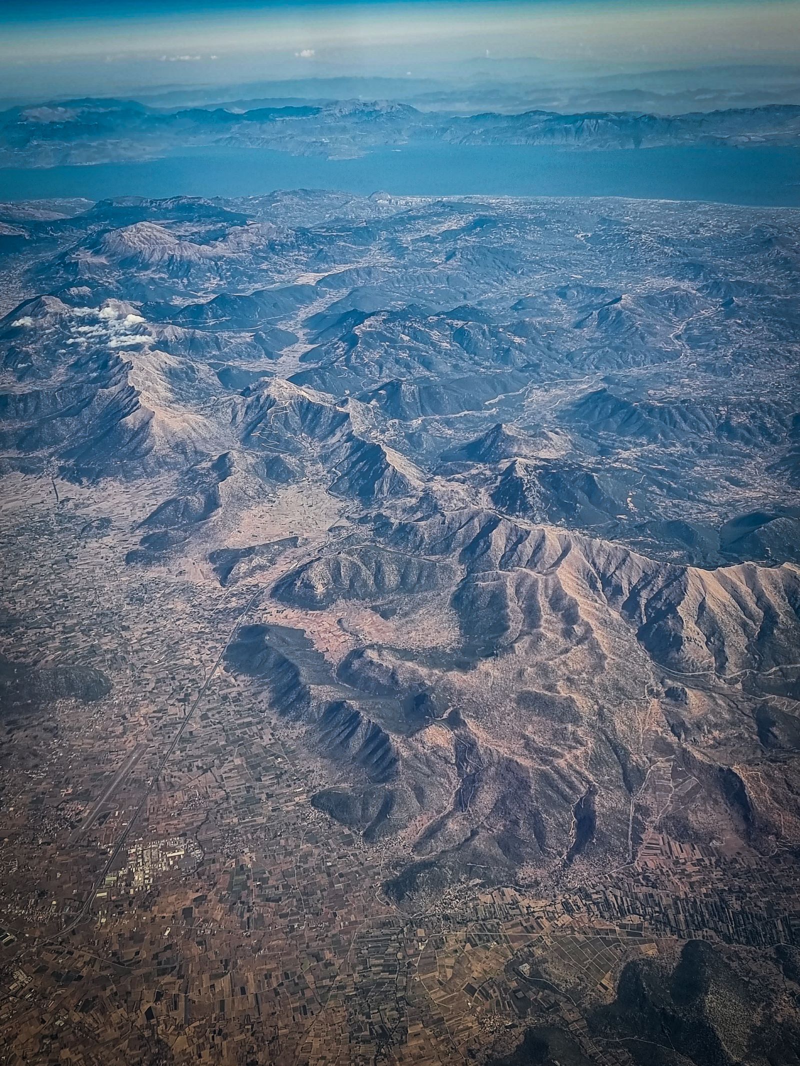
Photo: Francesco Ungaro / Pexels
Set the Sun on Purpose: The Hillshade Checklist
Check off each step as you finish it. Your progress stays on this page.
0 of 8 complete
0% done
What a Hillshade Is, and Is Not
A hillshade is a visualization, not a measurement. It encodes no elevation values you can query; it encodes slope and aspect, the steepness and facing direction of each cell, rendered as brightness under an imaginary sun. That is why it pairs so well with the DEM itself: draping a semi-transparent hillshade over a color-ramped elevation layer gives you both channels at once, color for height, shading for shape, which is the standard look of professional terrain maps. It is also why a hillshade alone can mislead: flat valley floors and flat plateaus shade identically, north-facing and south-facing slopes of a symmetric ridge differ only by the light you chose, and nothing in the image tells you whether the terrain rises a hundred meters or ten. Treat it as the DEM's portrait, not its data. If you need actual numbers along a route, that is the job of an elevation profile; the hillshade's job is to make the country's shape legible at a glance, for map readers, for site selection, and for spotting landforms, old shorelines, fault scarps, archaeological earthworks, that flat ramps conceal.
Make One: The Standard Recipe
Load a DEM, a digital elevation model raster covering your area; public sources and download routes are covered in our guide to downloading data from The National Map. In QGIS, open Processing, then Raster terrain analysis, then Hillshade. The defaults are the cartographic convention refined over a century of Swiss mapmaking: azimuth 315 degrees, the sun placed in the northwest, and altitude 45 degrees, the sun halfway up the sky. Leave the Z factor at 1 for now if your DEM is in a projected CRS with meter units, a condition the next sections interrogate, and run. The output is a grayscale raster, dark in the shadowed slopes, bright on the lit ones. Style it for real use: set the layer to a partial transparency and place it above your elevation layer rendered with a color ramp, or above a plain background for a relief-only map. That three-minute product, DEM plus hillshade overlay, is the terrain base underneath most of the maps in this site's guides, and for most purposes you are done. The refinements below matter when the defaults misbehave or when the terrain is subtle.
Azimuth and Altitude: What the Two Numbers Mean
Azimuth is the compass direction the light comes from, measured clockwise from north. The 315-degree default, northwest light, is convention with a reason: humans read relief most naturally when light falls from the upper left of the page, and northwest light on a north-up map does exactly that; flip the sun to the southeast and the terrain appears inverted, valleys reading as ridges, a famous optical trap that has embarrassed real publications. Altitude is the sun's height above the horizon: lower sun, 30 degrees or less, rakes across the land and exaggerates small relief, which is why archaeologists hunting faint earthworks choose low angles, while a high sun near 60 degrees flattens and clarifies. Change one variable at a time and re-render; hillshade is cheap. QGIS also offers a multidirectional mode, which lights the terrain from several azimuths at once and removes the directional bias entirely: no slope direction goes dark just for facing away, which makes it the better analytical backdrop, at the cost of some of the classic portrait drama. For a map meant to be read, single-direction northwest remains the default for a reason; for terrain you intend to measure with your eyes, multidirectional is the honest choice.
The Z-Factor Trap
Now the failure that produces the melted-wax and lunar landscapes. The hillshade computation compares vertical change against horizontal distance, so both must share units. If your DEM lives in a geographic CRS, its horizontal units are degrees while its elevation is meters, and a degree of longitude is roughly a hundred thousand meters, so the math, left uncorrected, sees terrain a hundred thousand times flatter or steeper than reality depending on direction of the error, and renders accordingly. The Z factor is the correction: a multiplier converting the vertical units into the horizontal ones. For a meter-elevation DEM in degrees, the standard remedy is a Z factor around 111320 scaled by the cosine of latitude, the figure GIS documentation commonly supplies, or, more robustly, reproject the DEM into a projected CRS with meter units before shading, which removes the mismatch entirely and improves every other terrain analysis you will run on it. Our reprojection guide walks that conversion. The diagnostic habit: when a hillshade looks absurd, ask first what units the DEM's CRS uses. Nine times in ten the answer explains the picture, and the fix is a number, not an afternoon.
Make It Read Better
With a correct base render, three refinements separate adequate from excellent. First, resampling and scale: a hillshade computed from a very fine DEM at a small map scale turns to noise, every plow line shouting; aggregating the DEM or softening the shading restores the landforms that matter at your scale. Second, blending: instead of plain transparency, experiment with the hillshade layer's blend mode, multiply over a muted elevation ramp is the classic, so colors stay clean and shadows deepen naturally. Third, pairing with slope: areas too steep to build, farm, or cross can be tinted from a slope raster while the hillshade carries the shape, a combination land managers use daily. Resist the urge to over-process. The hillshade's power is that a reader understands it with no legend and no training, and every cleverness that survives should be one that keeps that instant readability intact. Make the standard one first, look at it with fresh eyes, and only then tune.
Hillshade in Practice: Three Jobs It Does Quietly
Close with the work hillshades actually perform once they hang in a project, because the use cases explain the settings better than theory does. In site selection, a hillshade over a cadastre or a road network reveals the terrain logic a flat map hides: which parcels sit on benches, which road alignment fights a side slope, where a proposed path will spend its life in a gully; planners read these in the shading before a single contour is consulted. In landform detective work, archaeology is the famous case, lidar-derived hillshades at low sun angles exposing earthworks, hollow ways, and field systems invisible on the ground, but the same eye serves geologists tracing fault scarps and old landslide bodies, and ecologists reading the drainage texture that decides habitat. In communication, the hillshade is the layer that makes a technical map legible to a non-technical audience: put relief under a zoning proposal or a trail plan and the room understands the country before the legend is read, which is why public consultation maps reach for it instinctively. Each job tunes the recipe: communication wants the classic northwest portrait, detective work wants low sun and several azimuths, analysis wants the multidirectional neutrality. The tool is one dialog; the craft is knowing which sun your question needs, and that craft is mostly what this guide has been teaching under the cover of two angles and a correction factor.
Printing and Presenting Relief
A hillshade that sings on screen can die on paper, so presentation deserves a closing word. In print, keep the base colors pale and let the gray do the talking; saturated fills that looked rich on a monitor flatten relief in ink, and a slightly stronger contrast in the shading itself survives the transition better than bold colors do. At small sizes, the finest terrain detail turns to noise, so for a small-format map, generate the hillshade from a generalized DEM or accept a softer rendering rather than shrinking a detailed one into static. In presentations and reports, label the hillshade's source and cell size in the figure note, because relief derived from a national DEM and relief from a global model are different evidence, and your audience deserves to know which they are admiring. Exported for another designer, the hillshade travels best as a grayscale raster with its world file, composited at their end, rather than baked into a flattened image nobody can re-tint. These are finishing habits, but relief is usually the layer a map is remembered by, the one that makes a reader say the country looks real. Finishing it properly is not vanity; it is the difference between evidence that persuades and evidence that merely decorates.
Related Guides
If this page answered part of the question, these GIS and open map data guides cover the rest of the same ground:
- Geocoding in QGIS: Turn a Table of Addresses Into Points With MMQGIS: Every spreadsheet of addresses is a map waiting to happen, and geocoding is the machine that makes it: street, city, and country in, points on the...
- New Layer From Selection in QGIS: Turn Chosen Features Into Their Own Dataset: A selection is an answer, but it evaporates: close the project, clear the highlight, and the features you so carefully isolated are anonymous again.
- QGIS Field Calculator: Build and Fix Attributes With Expressions: The Field Calculator is where a QGIS layer's attribute table becomes programmable: an expression engine that can create new fields, update...
- QGIS Raster Calculator: Band Math, Worked Expressions, and the Nodata Traps: expressions beyond a single hillshade
- Viewshed Analysis in QGIS: What a Point Can Actually See: The DEM as evidence instead of picture: line of sight from a point.
Frequently Asked Questions
What do the default hillshade settings in QGIS mean?
Azimuth 315 degrees places the imaginary sun in the northwest, the cartographic convention that makes relief read naturally on a north-up map. Altitude 45 degrees puts the sun halfway up the sky. Z factor 1 assumes your DEM's horizontal and vertical units already match, typically both meters.
Why does my hillshade look melted or absurdly rugged?
Almost always a unit mismatch: the DEM is in a geographic CRS with degree units horizontally and meters vertically. Set a Z factor that converts between them, around 111320 adjusted for latitude, or reproject the DEM to a projected CRS in meters and shade that instead.
Is a hillshade the same as elevation data?
No. A hillshade is a picture of how terrain would look under angled light; it encodes slope and aspect as brightness, not elevation values. Query the DEM itself for heights, and drape the hillshade over a colored DEM to read height and shape together.
What is multidirectional hillshade?
A mode that lights the terrain from several directions at once, so no slope goes dark merely for facing away from a single sun. It removes directional bias and suits analytical backdrops, at the cost of the classic single-light portrait look.
Which sun angle is best for subtle terrain like archaeology?
A low altitude, around 30 degrees or less, rakes light across the ground and exaggerates faint relief such as earthworks and old field systems. Trying a couple of azimuths also helps, since a feature aligned with the light can vanish from one direction and pop from another.
Photo credits: Francesco Ungaro (Pexels); Josh Withers (Pexels). Photos are served from this site; follow the credit to the library page for the original.