Every raster in your project is a grid of numbers wearing a picture as a disguise. The Raster Calculator is the tool that works on the numbers directly. Give it an expression, arithmetic over one band or several rasters, and it writes a new grid whose every cell is the expression evaluated at that spot. With it you build vegetation indices from satellite imagery, threshold a DEM into flood levels, combine layers into suitability scores, and reclassify continuous data into the categories a decision needs. It is also, in the experience of everyone who teaches QGIS, the tool whose failures are quietest: a wrong extent, a nodata leak, a band referenced by the wrong name, and the output looks plausible while being wrong. This guide teaches the tool the way careful practitioners use it: the interface, the syntax, a fully worked example, and then the traps, because the traps are the curriculum.
Home / GIS and Open Map Data for Beginners
QGIS Raster Calculator: Band Math, Worked Expressions, and the Nodata Traps
Photo: Tony Wu / Pexels
Grid Math, Checked Twice: The Raster Calculator Checklist
Check off each step as you finish it. Your progress stays on this page.
0 of 7 complete
0% done
The Interface and the One Syntax That Matters
Find the tool at Raster, Raster Calculator. The dialog has three territories: the list of your loaded rasters, the expression box, and the output settings. Double-clicking a raster in the list inserts its reference into the expression, and that reference is the one piece of syntax everything else hangs on: "layer name@band number", as in "sentinel@1". The quotes carry the layer name, the @ picks the band, so a four-band image offers @1 through @4 and a DEM, a single band, is simply @1. Around that reference you write ordinary arithmetic, +, -, *, /, parentheses, comparison and logical operators, and functions including the conditional IF, written as IF(condition, value if true, value if false). The discipline that saves beginners is to build expressions by double-clicking references rather than typing them: a typed reference with a typo fails loudly if you are lucky and silently references nothing if you are not, while an inserted reference is guaranteed to name a band that exists. Set the output file and format deliberately too, GeoTIFF unless you have a reason otherwise, and let the calculator take its extent and resolution from a reference layer you choose, a setting the next sections will show is not a detail but a decision.
Worked Example: NDVI From Two Bands
The canonical calculator job is NDVI, the normalized difference vegetation index, computed from a satellite image's near-infrared and red bands as (NIR - Red) / (NIR + Red). Healthy vegetation reflects near-infrared strongly and absorbs red, so the index runs toward 1 for dense green growth and toward 0 or below for bare soil, water, and concrete. With a four-band image whose first band is red and fourth is near-infrared, the expression reads:
("image@4" - "image@1") / ("image@4" + "image@1")
Check the arithmetic by hand on two pixels before you trust the grid. A vigorous crop pixel with NIR at 0.50 and red at 0.08 gives (0.50 - 0.08) / (0.50 + 0.08) = 0.42 / 0.58, which is about 0.72, deep in healthy territory. A stressed pixel with NIR at 0.30 and red at 0.25 gives 0.05 / 0.55, about 0.09, essentially bare. Run the expression, then interrogate the output at pixels whose land cover you know: a forest, a field, a reservoir. The reservoir should sit near zero or negative. If your known water reads 0.7, the bands are not what you assumed, and you have caught the classic error, band order varies by sensor and by file, before it poisoned a report. The calculator computed faithfully; it computed the wrong bands. Verification against known ground is not paranoia. It is the method.
Extent, Resolution, and CRS: The Alignment Contract
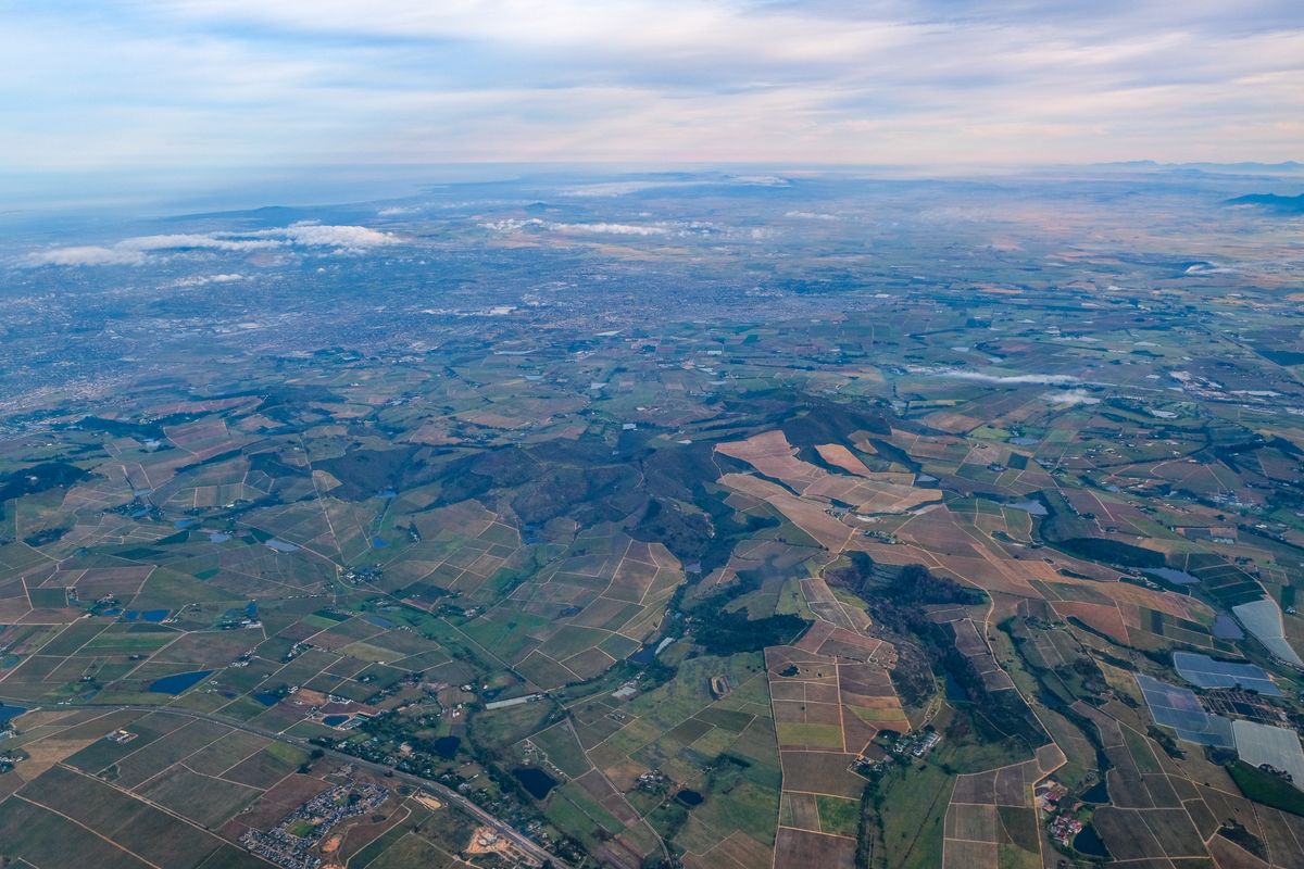
Raster math is cell-by-cell, which imposes a contract the calculator will not enforce for you: the inputs must align. Same extent, same cell size, same CRS, or the expression pairs cells that do not describe the same ground and the output is fiction with good formatting. The dialog lets you set the output extent and resolution, by typing values or taking them from a selected layer, and the professional habit is to choose your most important input as the reference and align everything to it. When inputs genuinely differ, a DEM at 30 meters against imagery at 10, resample deliberately with the warp and align tools first, and know that resampling is an interpretation, not a copy: nearest neighbor for categories, bilinear for continuous surfaces. CRS mismatches are the sneakiest version, because two rasters can look stacked in the canvas, thanks to on-the-fly reprojection, while their native grids disagree entirely. The canvas forgives. The calculator does not. Check the layer properties, not the picture, and align the data before the expression, every time.
Nodata: The Silent Partner in Every Expression
Every real raster has nodata cells: the border outside the flight lines, the cloud the provider masked, the ocean in a land dataset. The calculator propagates nodata honestly in principle, a nodata input makes a nodata output, but the edges of that honesty are where sessions go wrong. Expressions involving comparisons and IF can resurrect nodata into numbers if the condition routes around it, and division invites the second classic failure: a denominator of zero, which NDVI dodges because NIR + Red is rarely zero, but ratio and change-detection expressions meet constantly. Defensive expression writing is a learnable style. Guard denominators by adding a tiny constant or by wrapping the whole expression in an IF that assigns a deliberate value where the denominator is zero. Decide what nodata should mean in your output before you run, then verify afterward: open the output's properties, read its actual minimum and maximum, and compare them against the range your expression could legitimately produce. An NDVI grid claiming a maximum of 4.2 has told you, in numbers, that something upstream is wrong. Listen to it. When the analysis matures from one grid to summaries over farms, districts, or watersheds, the natural next tool is zonal statistics, which reads a calculator output the way this tool reads bands.
Chaining, Reclassifying, and Knowing the Neighbors
Real work chains expressions. A slope raster from a DEM feeds a threshold expression, buildable land where slope is under a chosen grade; the IF function turns continuous outputs into decisions, IF("slope@1" < 8, 1, 0), and a weighted sum of normalized layers builds the suitability map a planning meeting argues over. Two habits keep chains honest. Save each intermediate with a name that states its content and units, because a folder of output1, output2, and final_real.tif is a future misunderstanding. And keep the expressions themselves: paste them into a text file with the project, since the calculator remembers nothing for you, and the colleague who must reproduce your flood map next year needs the recipe, not just the cake. Know the tool's neighbors too, so you reach for the right one: clip raster cuts grids to a boundary before or after math, hillshade is a specialist expression the calculator could write but should not have to, and the expression builder is the vector-side cousin of this dialog, same philosophy, different data. The raster calculator remains the center of grid work: one expression, honestly aligned, verified against ground you know.
Four Expressions That Earn Their Keep
Beyond NDVI, a working vocabulary of expression shapes covers most of what the calculator is asked to do, and each teaches a habit. The threshold: IF("dem@1" < 12, 1, 0) paints every cell below 12 meters with 1 and everything else with 0, a flood-plain mask from a DEM in one line, and the ancestor of a hundred planning arguments. The slope mask: run the slope tool first, then IF("slope@1" < 8, 1, 0) separates the ground a project can use from the ground it cannot, and chaining the two outputs is the calculator's normal working rhythm. Change detection: subtract last decade's index grid from this year's, ("ndvi_2025@1" - "ndvi_2015@1"), and the difference grid reads as a map of gain and loss, provided the two inputs were aligned and radiometrically comparable, the alignment contract doing its quiet work again. The weighted suitability sum: normalize each factor grid to a common 0 to 1 scale, then add them with weights that sum to 1, as in 0.5 "slope_score@1" + 0.3 "water_dist@1" + 0.2 * "road_dist@1", and the output is an argument made visible, every assumption exposed in the weights where a committee can argue with it. Keep these four shapes in your project notes with the band references adapted to your data. Most raster careers are variations on them, and the variations go better when the originals were written carefully, verified against known ground, and saved where the next analyst can find them.
Temporary Answers, Permanent Ones: Managing Outputs
The calculator produces two kinds of output, and confusing them is a rite of passage best shortened by reading about it. A temporary output lives in scratch memory for the session: perfect for the intermediate steps of a chain, the slope mask you will feed into the next expression, the experimental index you may discard by lunch. Its virtue is speed and its vice is mortality; close the project and it is gone, taking any layer styled from it into honest oblivion. A saved output is a real file at a real path, and it deserves the full ceremony: a name that states the recipe and the inputs (ndvi_2025_s2_l2a says more than output3 ever will), a folder that separates raw inputs from derived products, and, for the outputs that will be cited, a line in the project notes recording the expression verbatim. The working rhythm this produces is unglamorous and effective: chain intermediates as temporary layers while you think, save the survivors with honest names when the thinking settles, and never let a temporary layer become a load-bearing part of a deliverable. Add one environmental habit: know your project's default output format and compression, because a season of uncompressed float grids will fill a disk with the confidence of a rising river, and the calculator will not warn you. It assumes, as it assumes everywhere, that the analyst is managing the workshop while it manages the math.
Related Guides
Readers working through this topic usually need its closest companions too. These GIS and open data guides cover the neighboring ground:
- QGIS Zonal Statistics: Summarize a Raster by Polygon Zones: The natural next step: turn the grid this tool produces into one row of statistics per farm, district, or watershed.
- QGIS Clip Raster: Cut Imagery and DEMs to Your Boundary With a Mask Layer: Cut grids to your study area before or after the math, so the calculator only computes ground you care about.
- QGIS Hillshade: Turn a DEM Into Readable Terrain, and Fix the Z-Factor Trap: The specialist neighbor: a canned expression for terrain shading, and what its settings really do.
- QGIS Expression Builder: The One Dialog Behind Selection, Fields, and Styles: The vector-side cousin of this dialog, where expressions compute fields instead of grids.
- Kriging in QGIS: Interpolation With a Semivariogram, and When IDW Is Enough: Building the surfaces the calculator computes on, with the variance map IDW cannot draw.
Frequently Asked Questions
How do I reference a band in the Raster Calculator?
With the syntax "layer name@band number", for example "dem@1" for the first band of a layer named dem. Double-click the layer in the calculator's list to insert the reference rather than typing it, so the name and band always exist.
Why does my NDVI output look wrong?
Most often the band order is not what you assumed: sensors and files order red and near-infrared differently. Check the output at places you know: water should sit near zero or negative, dense vegetation high. If known water reads as vegetation, swap the bands.
What happens when my rasters have different extents or resolutions?
The calculator pairs cells positionally, so misaligned inputs produce plausible fiction. Align everything to a chosen reference first: same extent, cell size, and CRS, resampling deliberately where the data genuinely differs.
How do I avoid division by zero errors?
Guard the denominator: add a tiny constant where it is safe, or wrap the expression in an IF that assigns a deliberate output value wherever the denominator is zero. Then check the output's real minimum and maximum against the range your expression could legitimately produce.
Can the Raster Calculator reclassify a raster?
Yes. Comparisons and the IF function turn continuous values into categories: IF("slope@1" < 8, 1, 0) writes a binary grid of buildable and unbuildable cells. Chain expressions like this, saving each intermediate with a name that states its content.
Photo credits: Tony Wu (Pexels); Magda Ehlers (Pexels). Photos are served from this site; follow the credit to the library page for the original.