A topographic map is a promise: that height has been made legible. The walker reads a slope from shading before a single contour is traced; the planner trusts the tint sequence to mean ascent in the same order everywhere on the sheet. QGIS can keep that promise with parts it already ships, a digital elevation model, a hypsometric tint ramp, a hillshade, contours, and the print layout, but the parts do not assemble themselves, and the tutorials scatter the order across a dozen pages. This guide is the assembly in one place: the stack, bottom to top, the blend that makes relief read as relief, contours extracted so their labels can speak, and the layout finish that turns a terrain view into a sheet. Two handoffs bound the scope honestly. The hillshade as a product in itself, its azimuth, altitude, and Z-factor discipline, is owned by our hillshade guide; the skill of reading a finished topographic map belongs to the map-reading guide. Here, the making is the subject.
Home / GIS and Open Map Data for Beginners
QGIS Topographic Map: From DEM to a Finished Sheet

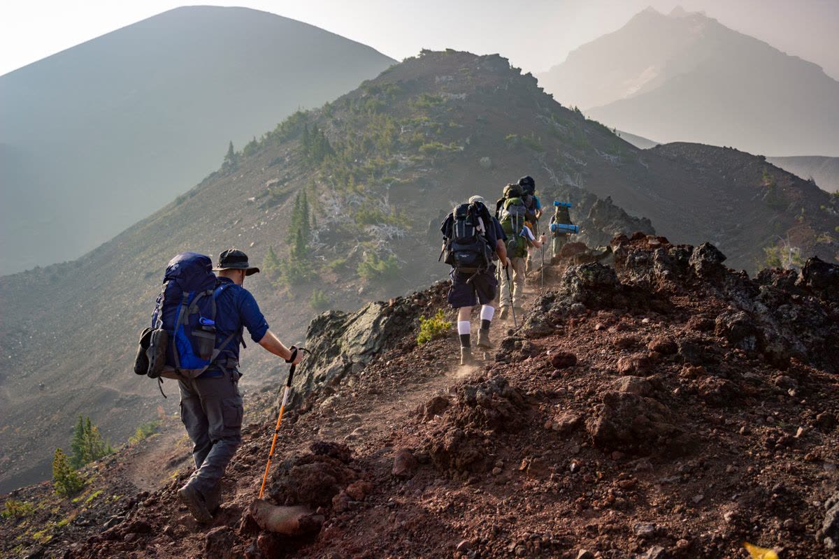
Photo: Sindre Fjerdingby Korsviken / Pexels
Build the Sheet in Order: The Topographic Checklist
Check off each step as you finish it. Your progress stays on this page.
0 of 7 complete
0% done
Start With the DEM, and Judge It
Everything stands on the digital elevation model, and the first professional act is judging the one you have. Its resolution sets the finest terrain the map can honestly show: a 30-meter DEM cannot draw a footpath's cutting, and contours finer than the grid are decoration lying about precision. Its projection should be a projected CRS in meters before any slope or contour work, because terrain math in degrees produces numbers with no meaning. Its voids and edges matter at the sheet's margins, where a DEM that ends mid-slope draws a cliff the world does not contain. Sources such as the SRTM and Copernicus elevation families cover most of the earth at useful resolutions, distributed as tiles that the GDAL tools mosaic and clip to your sheet's extent, work our GDAL guide covers at the library level. Clip generously beyond the neatline, so the hillshade's light has terrain to fall on at the edges, and keep the unclipped mosaic: the next sheet in the series will want it.
The Stack: Tint, Shade, Slope
The classic relief stack has three layers in a deliberate order. At the bottom, the hypsometric tint: the DEM itself, styled with a color ramp that climbs with elevation, greens in the lowlands through yellows and browns to pale heights, or a restrained local scheme of your own, applied as a smooth gradient so elevation reads as a continuous field. Above it, the hillshade, the simulated light across the terrain, set to a multiply blend mode in its layer blending settings: multiply darkens the tint where the modeled slopes fall away from the light and leaves the lit slopes' colors clean, which is the entire trick of shaded relief, color carrying the height, shading carrying the shape. Above those, where the terrain and the audience justify it, a slope layer can emphasize steepness for hazard or engineering readers, usually kept subtle or omitted for a general sheet. Each layer alone is a dataset; blended in this order they are a landscape. The judgments live in the ramp and the shade: a ramp whose steps argue with the contour interval confuses, and a hillshade too strong turns the sheet into a photograph of a model. Our hillshade guide owns the shade's own parameters, azimuth, altitude, and the Z-factor trap that exaggerates or flattens relief when units mismatch; here it is enough to know the shade is a guest in the tint's house, and multiply is the etiquette that keeps it polite.
Contours: Extraction With Labels in Mind
Contours are the sheet's contract of precision, and in QGIS they come from Raster, Extraction, Contour, run on the DEM. Two decisions at extraction time determine whether the finished sheet reads well. The interval should match the DEM's honest resolution and the sheet's scale: too fine and the map is spaghetti, too coarse and the terrain's character vanishes; index contours, every fifth line, drawn heavier, give the reader the ladder the labels climb. And the extraction should write an elevation attribute field on the contour lines, because that field is what the labels will print: contour labels drawn from the attribute, placed along the lines with the label engine's curved placement, are how a reader learns a valley's height without hunting a legend. Style the lines themselves with restraint, a muted brown or gray that sits above the tint without shouting over it, index lines stronger, and let the labels, sparse and upright-readable, do the numeric work. A sheet whose contours carry no labels is a picture; a sheet whose labels sit on an elevation attribute is an instrument.
Drainage, Names, and the Honest Furniture
A topographic sheet earns its name with more than relief. Water is the walker's second language: streams and lakes in a clear blue, drawn from hydrography data or OpenStreetMap extracts, sitting above the tint and below the contours in the stack's social order, because water explains valleys the shading only suggests. Place and feature names follow the label engine's hierarchies: settlements, peaks with their spot heights, passes, the named furniture by which a reader navigates from map to ground. Spot heights and benchmarks, where data provides them, punctuate the contour story with surveyed certainty. The discipline across all three is hierarchy: each element's weight on the sheet should match its weight in the reader's decisions, and the relief, the sheet's reason to exist, stays visually in charge. It is easy to keep adding layers until the map is a database wearing a neatline; the topographic tradition is the opposite art, a selection.
The Layout Finish
The sheet becomes a sheet in the print layout: the map frame at a declared scale, a neatline, a title that names the country of the map rather than its author, a scale bar in the units the audience walks in, a north arrow verified against the frame, and the margin notes that make the sheet citable: the DEM's source and resolution, the contour interval, the projection, the date. Our rotate guide covers the frame's orientation decisions, including the classic move of turning the sheet so a diagonal range runs with the page. Proof the export at full size and at arm's length: relief that reads beautifully at screen zoom can flatten in print, and contour labels that seemed sparse on screen can crowd at paper scale. The layout is also where the series discipline lives: a second sheet from the same stack, tint ramp, and furniture will match the first, and a wall of matching sheets is the quiet signature of a mapping program rather than a mapping afternoon.
The Workflow, Compressed
DEM judged and projected; mosaic clipped wide. Tint ramp applied to the DEM, smooth and legible. Hillshade generated, blended on multiply, strength restrained. Slope consulted, kept only if it earns its place. Contours extracted at an honest interval, elevation attribute written, index lines weighted, labels placed from the attribute. Water and names layered with hierarchy. Layout: frame, scale, neatline, north, and the margin's honest credits. Every step exists in QGIS's standard toolkit, and the order is the content: relief first as a blended field, precision second as labeled lines, meaning third as furniture, and publication last as a sheet. That order, kept, produces topographic maps that a stranger can trust, which is the only kind worth making.
The Ramp Is an Argument
The hypsometric ramp deserves a slower look, because it is the sheet's thesis about the land. A good ramp is perceptually ordered: each step must read as higher than the last at a glance, in color and in lightness together, which is why the classic green-to-brown-to-white sequence survives, it climbs in the reader's intuition as well as in elevation. It is matched to the terrain's own distribution: a sheet of low hills wants its ramp's drama concentrated in the low bands where the land actually lives, while an alpine sheet spends its palette at altitude, and a ramp stretched evenly over elevations the map barely contains wastes its voice on empty octaves. It is print-honest: colors chosen on a backlit screen will be judged on paper, in photocopies, and under field light, so the ramp must keep its order in grayscale and survive a bad printer without its steps collapsing into one another. And it is consistent across the series, because a reader who learns your ramp on one sheet should be able to spend that learning on the next. Treat the ramp as typography for height: chosen once, with reasons, and then left alone to become a convention your readers can trust.
Sources for the Furniture
The relief is derived; the furniture is gathered, and its sources deserve the same skepticism as the DEM. OpenStreetMap extracts supply roads, water, settlements, and names for most of the earth, at a completeness that varies by region and must be eyeballed against the imagery before it is trusted on a sheet. National mapping and hydrography datasets serve where they are open, with an authority community data cannot always match. Gazetteers and peak registers settle names and summit elevations that a DEM can only estimate, since a grid's highest cell is a sample, not a surveyed summit. The margin notes are where these debts are declared: a sheet that credits its DEM, its water, and its names is a sheet a professional can build on, and the crediting habit costs nothing but the decision to keep it.
A final production note: sheets in a series should share more than a stack. The same tint ramp, the same contour interval logic, the same furniture hierarchy and margin layout turn separate exports into an atlas, and the time to fix those choices is on the first sheet, when changing them is free, rather than on the fifth, when it means redoing four.
Related Guides
If this page answered part of the question, these GIS guides cover the rest of the same ground:
- QGIS Hillshade: Azimuth, Altitude, and the Z-Factor Trap: The shade as a product in itself, handed its depth there.
- How to Read a Topographic Map: The reader's side of the sheet this guide teaches you to make.
- QGIS Rotate Map: Canvas Rotation, Layout Rotation, and the Grid Rules: The frame orientation decisions a diagonal range demands.
- QGIS and GDAL: The Library Under the Hood: The mosaic and clip machinery under the DEM work.
Frequently Asked Questions
What data do I need to make a topographic map in QGIS?
A digital elevation model covering your area, in a projected CRS, at a resolution honest for your scale. Everything else, tints, hillshade, contours, is derived from the DEM inside QGIS; water and place names come from vector data such as OpenStreetMap extracts.
How do I blend the hillshade with the elevation colors?
Style the DEM with a hypsometric color ramp, generate the hillshade as its own layer above it, and set the hillshade layer's blending mode to Multiply. The tint carries height as color; the shade darkens slopes facing away from the light, so shape reads through the color.
How are contour labels produced?
Extract contours with the Raster Extraction Contour tool and have it write an elevation attribute field on the lines. Labels are then drawn from that attribute with the label engine, placed along the lines, so each labeled contour states its own height.
What contour interval should I choose?
One matched to the DEM's resolution and the map's scale: fine enough to show the terrain's character, coarse enough to stay legible. Intervals finer than the DEM's grid imply precision the data does not have.
Is a hillshade the same as a topographic map?
No. A hillshade is one layer, simulated light on terrain. A topographic map is the assembly: tinted relief, labeled contours, water, names, and the layout furniture that makes the sheet measurable and citable.
Photo credits: Sindre Fjerdingby Korsviken (Pexels); Eric Sanman (Pexels). Photos are served from this site; follow the credit to the library page for the original.