For most of its life, QGIS treated LiDAR the way a word processor treats spreadsheets: politely, through conversion, at arm's length. You turned your LAS files into rasters or shapefiles somewhere else and brought the corpses in. That era is over. Since QGIS 3.18, point clouds are a native layer type, loaded, rendered, styled, and processed inside the application, and the versions since have kept building: COPC and virtual point cloud (VPC) support in current releases, a 3D viewer that treats clouds as citizens, and a Processing toolbox with dedicated point cloud groups. This guide teaches the native workflow as it exists now: loading, the format menagerie, styling, 3D, and processing, with the data sources that feed it.
Home / GIS and Open Map Data for Beginners
LiDAR in QGIS: Native Point Clouds From LAS to 3D

Photo: Ella Wei / Pexels
Interactive tool
Points, Not Pixels: The LiDAR Checklist
Check off each step as you finish it. Your progress stays on this page.
0 of 7 complete
0% done
The Formats, Untangled
Point cloud files arrive in a small zoo of formats, and QGIS's handling of each is the first thing to know:
- LAS: the industry standard, uncompressed, the raw exchange format of the LiDAR world.
- LAZ: LAS compressed, the form most data actually ships in, often a tenth the size.
- EPT: Entwine Point Tiles, a tiled, indexed, streamable organization of a cloud. QGIS's internal preference: when you load a LAS or LAZ file, QGIS converts it to EPT on first load, building the index that makes pan and zoom over billions of points survivable. The conversion is a one-time cost per file; keep the generated EPT beside the source and subsequent loads are fast.
- COPC: Cloud Optimized Point Cloud, a modern single-file format with the index built in, designed for streaming and partial reads, supported in current QGIS.
- VPC: a virtual point cloud, a lightweight file that references many tiles as one layer, the way a mosaic references rasters.
Loading runs through the Data Source Manager's Point Cloud tab, the same front door as every other data type, which is the statement the feature makes: a point cloud is a layer now, not an import project.
The 2D View: Styling a Cloud Flat
On the map canvas, a point cloud renders as its points, and the symbology choices are the analyst's first questions made visible:
- Classification: color by the ASPRS class codes the data carries, ground, vegetation, building, water, and the map becomes a land-cover argument: this is the view that shows whether the classification your analysis depends on is any good.
- Elevation: a color ramp over height, the fastest terrain read the cloud offers, and the view in which drainage, ridges, and the odd erroneous skyscraper point announce themselves.
- RGB: the stored color from aerial imagery draped on the survey, where the data carries it, the photorealistic view and the least analytical.
Point size, density behavior at zoom, and the eye-dome lighting effect that gives flat-rendered clouds their sculptural depth are all in the same panel. The working habit: classification first for data quality, elevation for terrain sense, RGB for communication, in that order, every time.
The 3D View: Where Clouds Justify Themselves
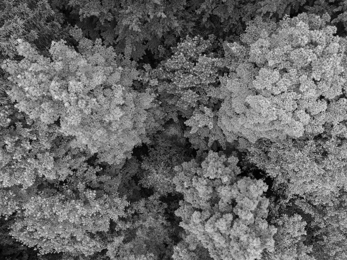
The 3D map view is where a point cloud stops being a dataset and becomes a place. QGIS's 3D view renders the cloud with its symbology, navigable by orbit and zoom, with the other layers of the project available around it. Foresters read canopy structure in it, engineers read clearances under wires and over roads, and everyone reads the one thing no raster conveys: the vertical arrangement of the world, trees over understory over ground, bridges over the water they cross. Performance follows the EPT and COPC indexing, which is why the first-load conversion matters: an indexed cloud streams its levels of detail as you move; an unindexed one makes you wait for its entirety. For big territories, build or obtain the cloud in tiles and bind them with a VPC, and the 3D view treats the mosaic as one terrain.
Processing: The Point Cloud Groups
The Processing toolbox carries dedicated point cloud groups, organized by intent: data management (assign CRS, build and convert between formats, merge and tile), extraction (clip by extent or polygon, filter by classification, height, or return), and conversion (to raster DEMs and DTMs, to vector). The standard products fall out of these groups in sequence: filter to ground classification, convert to a raster, and you hold the bare-earth DEM that feeds the watershed pipeline and the viewshed analysis, at resolutions aerial DEMs cannot match, with the buildings and canopy excluded by the classification filter rather than by hope. Long chains of these steps are exactly the work the Python console exists to script: parameterized, rerunnable, and indifferent to whether the territory is one tile or four hundred.
Getting Data: USGS First
Free LiDAR begins, for most readers, at USGS Earth Explorer and the national 3DEP program's holdings: point clouds for large and growing parts of the United States, downloadable as LAZ tiles with their metadata. State and regional portals add coverage and sometimes finer vintages. The download discipline mirrors the format lesson: take the LAZ, let QGIS build its EPT on first load, and record the survey's date and point density in your project notes, because a cloud is a measurement with a birthday, and the forest in it has been growing or falling since. Outside the US, national mapping agencies increasingly publish their airborne surveys openly; the search pattern is the country's name plus its mapping agency, and the prize is the same native workflow on home terrain.
Reading a Cloud: Returns, Density, and the Questions to Ask First
A point cloud is a measurement, and like every measurement it should be interrogated before it is used. Three questions, asked of the layer properties and the provider's metadata before any analysis, separate a survey you can build on from a pile of points. What is the point density? Points per square meter decides what the data can resolve: a sparse survey reads terrain and large structures honestly and invents the rest, while a dense urban survey supports building-level work. How many returns, and is the classification trustworthy? LiDAR pulses return multiple echoes, first return off the canopy top, last return likeliest to be ground, and the classification field records the processor's judgment about each point. Style by classification and look at the map before believing it: ground points floating above rooftops or building points buried in fields are the signature of a classification pass that needs skepticism, and every DEM downstream inherits whatever you accept here. When was it flown? The survey's date bounds every claim: a five-year-old cloud describes a forest five years younger, a shoreline five storms ago. None of these questions requires leaving QGIS; all of them are cheaper than the analysis they protect.
From Cloud to Contour: A Small Worked Path
The path most users actually travel deserves a walkthrough in words. Load the LAZ tiles for a study area through the Point Cloud tab and let the EPT indexing build. Style by classification and audit the classes against the aerial imagery you know: does the building class sit on buildings, does the ground class thread the valleys? Filter the cloud to ground points with the extraction tools, and convert that subset to a raster at a cell size the density can honestly support, a meter for dense surveys, coarser for sparse ones, because a fine grid over sparse points is interpolation wearing a survey's clothes. The result is the bare-earth DEM. Style it with hillshade, check the drainages against the map you trust, and the DEM is ready for the watershed and viewshed pipelines named above. Save each intermediate, cloud subset and raster alike, with names that state their recipe, ground-only, 1 meter, survey year, because in six months the folder is the only memory the project has, and a DEM whose lineage is guesswork is a liability wearing a result's clothes.
Honest Limits
Native does not mean magical. Clouds are big: a county survey can run to hundreds of gigabytes, and the EPT conversion, while one-time, is a real cost in time and disk. Classification quality varies by survey and vendor, and every analysis built on the ground class inherits its sins. And QGIS's point cloud tools, young beside its raster and vector depth, cover loading, styling, viewing, and the core processing well, while specialist classification and feature extraction still live in dedicated LiDAR software. The native workflow's claim is the one this guide has made: the common path, file to map to DEM to analysis, now runs entirely inside the free application, and that was not true five years ago.
Related Guides
If this page answered part of the question, these GIS and open data guides cover the rest of the same ground:
- The QGIS Python Console: Drive the Whole Application With Code: Scripting the conversion and filtering chains that point cloud work runs on.
- Rule-Based Symbology in QGIS: Styles Written as Conditions: The vector styling system, for the layers your clouds get analyzed alongside.
- Watershed Delineation in QGIS: From a DEM to a Basin Boundary: The main destination of a LiDAR-derived DEM: flow, accumulation, and the basin.
- Viewshed Analysis in QGIS: What a Point Can Actually See: Line of sight over terrain, where a LiDAR surface model changes the answer honestly.
Frequently Asked Questions
Can QGIS open LAS files directly?
Yes, since QGIS 3.18 point clouds are a native layer type. Load LAS or LAZ through the Data Source Manager's Point Cloud tab. On first load QGIS converts the file to EPT, an indexed tiled form, which makes large clouds responsive; the conversion happens once per file.
What is the difference between LAS, LAZ, EPT, and COPC?
LAS is the uncompressed standard; LAZ is its compressed form, how most data ships. EPT is a tiled, indexed organization QGIS builds for fast rendering. COPC is a modern single-file cloud-optimized format with indexing built in, supported by current QGIS versions. All four describe the same kind of data: points with attributes.
How do I make a DEM from LiDAR in QGIS?
Filter the point cloud to the ground classification using the Processing point cloud tools, then convert the filtered cloud to a raster. The result is a bare-earth DEM. Using all returns instead gives a surface model with buildings and canopy included; state which one you made.
Where can I get free LiDAR data?
USGS Earth Explorer is the main source for the United States, carrying the 3DEP program's point clouds as downloadable LAZ tiles. Many state portals and, increasingly, national mapping agencies abroad publish their airborne surveys openly as well.
What is a VPC file?
A virtual point cloud: a small file that references many point cloud tiles and presents them as a single layer, the point cloud analogue of a raster mosaic. It is the practical way to work with a survey delivered as hundreds of tiles.
Photo credits: Ella Wei (Pexels); Justin Wolfert (Pexels). Photos are served from this site; follow the credit to the library page for the original.