A scanned map knows nothing. It is a picture: pixels in rows, no coordinates, no scale, no place. Yet it may hold information no modern dataset has, the 1947 street grid, the pre-dam shoreline, the orchard before the subdivision. Georeferencing is the ceremony that marries such a picture to the Earth. You point at features in the image whose real positions you know, road junctions, survey markers, building corners, and QGIS computes a transformation that stretches the image onto the map. Done well, a century-old sheet lands within meters of its modern streets. Done carelessly, it lands in a confident, wrong place and poisons every analysis stacked on it. This guide walks the workflow in QGIS's Georeferencer and, more importantly, teaches the checking habits that separate the two outcomes.
Home / GIS and Open Map Data for Beginners
QGIS: How to Georeference an Image, From Scan to GeoTIFF
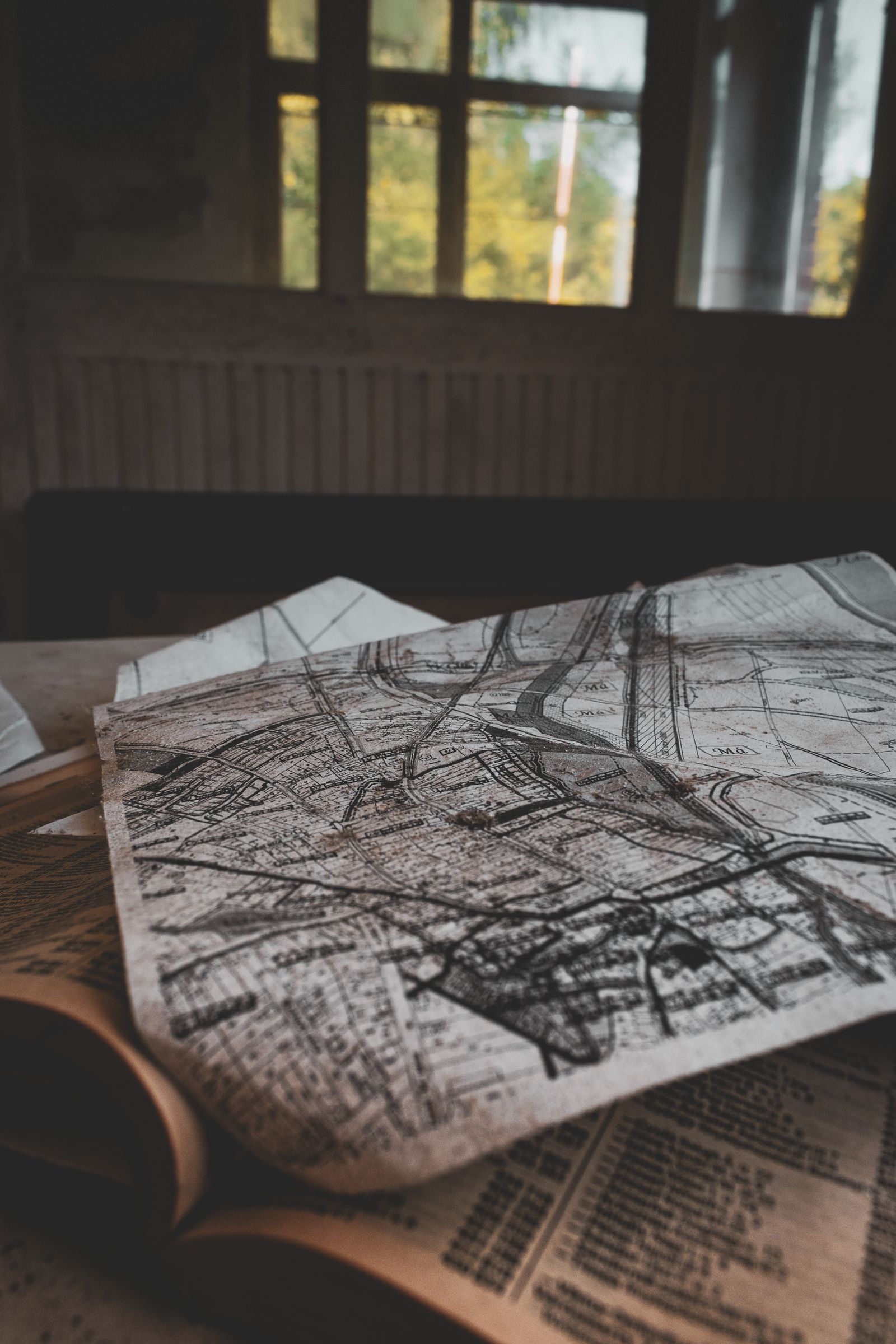
Photo: Sándor Skoda / Pexels
Georeference Without Lying to Yourself: The Checklist
Check off each step as you finish it. Your progress stays on this page.
0 of 6 complete
0% done
Before You Open QGIS: Get an Image Worth Placing
The transformation can only be as good as the picture and the references you feed it. Scan flat and square, at a resolution that keeps map lettering legible; a skewed scan from a phone photo introduces distortions a polynomial will happily bake into your map. Know the image's vintage and source, because your control points must be features that existed then and survive now: a road junction rebuilt in 1970 is a trap on a 1947 sheet, while a church corner, a rail crossing, or a coastline headland may be stable across the whole span. Set your QGIS project to the coordinate reference system you want the output in before you start, and load a modern reference layer, OpenStreetMap or a current aerial basemap, that you will pick target coordinates from. Our QGIS beginner tutorial covers project setup and basemaps if any of that is new; this guide assumes the map canvas behind the Georeferencer already shows the neighborhood your image belongs to.
The Georeferencer: Where It Lives and How It Thinks
Open the tool from the Layer menu: Layer, Georeferencer, in QGIS 3.26 and later (earlier versions parked it under Raster). Load your image with the Open Raster button and it fills the Georeferencer window, a small GIS of its own. The workflow inside is a loop: click a point on the image, then tell QGIS where that point is in the real world, either by typing coordinates or by clicking the corresponding spot on the main map canvas with the From Map Canvas button. Each such pair is a ground control point, a GCP, and they accumulate in a table at the bottom with two extra columns that matter enormously: the residuals, covered below. Before adding points, open Transformation Settings and make the decisions the next sections explain: the transformation type, the resampling method, and the output, a GeoTIFF in your target CRS, with compression if the sheet is large. Settings first, points second; changing the transformation later reinterprets every point you placed.
Choosing the Transformation: Match the Math to the Damage
The transformation is the function that warps image pixels into map coordinates, and QGIS offers a ladder of them. A linear (affine style) transformation shifts, rotates, and scales uniformly; it suits a clean digital image that is merely unlocated, like an exported map graphic. Polynomial 1 can also correct slight skew; Polynomial 2 and 3 bend the image progressively, absorbing the warps of old paper, imperfect scans, and camera tilt, at the price of demanding more control points and risking wild behavior outside them. Thin Plate Spline forces the image exactly through every GCP and bends locally between them, powerful for badly distorted sources and dangerous for the same reason, since an error in one point becomes a local mountain in the fit. The minimum GCP counts in QGIS's documentation anchor the ladder: Polynomial 1 needs at least 3 points, Polynomial 2 at least 6, Polynomial 3 at least 10, Thin Plate Spline at least 4. Treat those minima as legal floors, not targets; practice uses comfortably more, spread as the next section demands. For most scanned topographic sheets, Polynomial 1 or 2 is the honest workhorse; reserve the heavy artillery for sources that demonstrably need bending.

Placing Ground Control Points: Spread, Stability, and Surplus
Point placement is the craft itself, and three rules govern it. First, spread: points must enclose the whole area you care about, corners and edges included, because a transformation interpolates politely inside the points' embrace and extrapolates recklessly outside it; a cluster of perfect points in one corner leaves the far corner to imagination. Second, stability: pick features identifiable to the pixel in both worlds, the center of a road junction, the corner of a building that still stands, a bridge abutment; avoid anything that moves, riverbanks, tree lines, shorelines on soft coasts, and anything you are merely fairly sure about. Third, surplus: place more than the minimum, roughly one and a half to two times it, because surplus points are what turn the residuals from decoration into diagnostics, and they let you delete a bad point without falling below the floor. Add points in a deliberate circuit, corners first, then edges, then interior, and watch the table as you go; the moment a point lands, its residual starts testifying.
Residuals and Mean Error: Reading the Fit's Confession
Each GCP's residual is the distance between where the transformation puts that point and where you said it should be, in map units. The table shows them per point, and the panel reports the mean error across all points. Read the residuals like a confession, point by point, not as a single score. A healthy fit shows small residuals of similar size scattered without pattern. A single huge residual names a bad point: you misclicked, or the feature moved between the image's era and now; the cure is to fix or delete that point, never to add more points hoping to drown it. A pattern, large residuals all along one edge, says the transformation type is too stiff for the image's distortion, and stepping up a polynomial order is the honest response. And now the lesson this whole article leans on, earned from a worked georeference of a 1947 USGS sheet: a mean error of zero is achievable with Thin Plate Spline by construction, because that transformation passes exactly through every point, and it proves nothing whatsoever about the map between the points. A zero score can hide a badly placed map the way a memorized exam answer hides an unlearned subject. The next section is the antidote.
The Check That Matters: Points the Fit Never Saw
Verification must use evidence the fit did not consume. Hold out a few identifiable features from your GCP set, or identify fresh ones after the transformation: a junction here, a building corner there, spread across the sheet. Measure where the georeferenced image puts them against where the reference map says they are. Those check distances, not the residuals, are your map's real accuracy statement, and they are the numbers to record alongside the output: "checked at six independent points, within 4 to 9 meters" is a claim a colleague can use; "mean error 0.00" is a claim about arithmetic. If the checks fail in one region, the remedy is local honesty: add GCPs there if stable features exist, or document the weakness and keep analysis away from that corner. This discipline generalizes beyond georeferencing, and it is the same discipline this site's article on adding GPS coordinates to QGIS applies to tabular data: a dataset is placed when independent checks say so, not when the software stops complaining.
Saving, Output, and Living With the Result
Run Start Georeferencing and QGIS writes the warped image as a GeoTIFF in your target CRS, optionally loaded straight into the project, where it should land on the basemap like a transparency settling onto a light table. Inspect it at working zoom across the whole sheet, tracing a road that crosses the image edge to edge; a good fit keeps it continuous with the modern network at every junction, not just at your control points. Keep the GCP table with the project, QGIS can save the points to a file, because the next person to question this layer deserves your evidence, and because re-running with one point changed is a five-minute job only if the points survive. Name the output with its source and year, set its transparency for overlay work, and write down the check distances somewhere a future user will find them. A georeferenced image treated this way becomes infrastructure. Treated as a one-click trick, it becomes the layer everyone quietly distrusts.
Which Images Georeference Well, and Which Fight Back
Experience sorts source images into the willing and the stubborn. Willing: printed topographic and cadastral maps, surveyed plans, and vertical aerial photographs over stable terrain. They were made to a projection in the first place, their features are surveyed rather than sketched, and a modest polynomial returns them to the Earth within a few meters. Stubborn: oblique photographs, tourist and pictorial maps, very old charts whose survey basis is guesswork, and anything drawn before triangulation reached its region. An oblique photo has no single transformation that fixes it, because perspective is not a warp a polynomial speaks; it needs photogrammetric treatment, and forcing it through the Georeferencer produces a layer that is right at the control points and drunk between them. Pictorial maps lie on purpose for legibility. Pre-survey charts can be off by kilometers in ways that vary across the sheet. The professional response is calibration of ambition: georeference the stubborn ones for orientation and storytelling, label their accuracy honestly in wide numbers, and never let them carry measurements. Knowing which class your image belongs to before you place the first point is half the skill, and it is a judgment no software update will automate away.
Related Guides
Readers working through this topic usually need its closest companions too. These GIS and open map data guides cover the neighboring ground:
- QGIS Elevation Profile: Read the Terrain Along Any Line You Draw: The Elevation Profile panel in QGIS turns a drawn line into a terrain cross-section: distance along the bottom, elevation up the side, with the...
- The QGIS Georeferencer: Pin a Scanned Map to the Real World: A scanned historical map is a picture until you georeference it: teach QGIS a set of ground control points, places whose real coordinates you...
- QGIS Heatmap: The Renderer for a Picture, the KDE Algorithm for a Raster: QGIS offers two different things called heatmap, and choosing between them is the first skill: the heatmap symbology renderer draws a live density...
Frequently Asked Questions
Where is the Georeferencer in QGIS?
Under the Layer menu in QGIS 3.26 and later: Layer, Georeferencer. In earlier versions it lived under the Raster menu and sometimes needed enabling in the plugin manager. It opens as its own window where you load the image, add ground control points, set the transformation, and run the georeferencing.
How many ground control points do I need?
At minimum, the transformation's floor: 3 for Polynomial 1, 6 for Polynomial 2, 10 for Polynomial 3, and 4 for Thin Plate Spline. In practice, use half again to twice the minimum, spread over the corners, edges, and interior of the area you care about, on features stable between the image's era and today.
What does a residual mean, and how big is too big?
A residual is the distance between where the transformation places a control point and where you specified it, in map units. Judge it against your purpose: a historical overlay for interpretation tolerates meters; data you will measure from demands better. One residual far larger than the rest usually marks a misclicked or moved feature; fix or delete that point rather than adding more.
Why is a mean error of zero not proof of a good georeference?
Because some transformations, notably Thin Plate Spline, are constructed to pass exactly through every control point, making residuals zero by design regardless of what happens between points. Real accuracy is measured at independent check points the fit never used. Verify there before trusting the layer.
What output should I choose?
A GeoTIFF in your project's target CRS is the standard: it embeds the georeferencing so any GIS can place it. Add compression for large scans, save the GCP points file alongside it, and record your independent check distances in the layer's notes or metadata so the accuracy claim travels with the data.
Photo credits: Sándor Skoda (Pexels); Gül Işık (Pexels). Photos are served from this site; follow the credit to the library page for the original.